An Introduction and Visual Framing of the In(put)s and Out(put)s of R Shiny

There Are Plenty of Existing Shiny Resources

This post is by no means attempting to replace the wealth of information at shiny.rstudio.com and elsewhere. I regularly use the articles and the galleries there for both reference and inspiration. And there is the R Shiny Cheatsheet, which, like many cheatsheets, is most useful as a reference once you have a pretty solid understanding of the underlying material.

And, these days, almost everything I build with Shiny uses flexdashboard, and I wind up on the same post every time to refresh myself on how to go about incorporating Shiny components into that world. I particularly like the fact that, with flexdashboard apps, I can put the output definitions (server) right next to the actual output display (ui) without having to worry about “server” vs. “ui”…although I think there is real value in having a basic intuition about the “ui” (front-end) of the app versus the “server” (back-end) of the app, which is something that this post addresses!

In short, yes, there are lots of existing resources. This post is simply meant to be a useful addition to that overall corpus.

Let’s get to it.

Starting at the End

Ultimately, this is the “complete” diagram that I came up with:

If you’re thinking, “Um…well…duh!” then…great! First, that means it’s accurate. But, second, that means you’ve got intuition and clarity around Shiny that it took me a while to get to.

If you’re thinking, “Oh…interesting. That seems a lot simpler than I’d thought things were. Do tell me more!” Well, then it might be useful to build this one piece at a time and describe each piece as we go. And…there’s a little bit of a bonus observation at the very end.

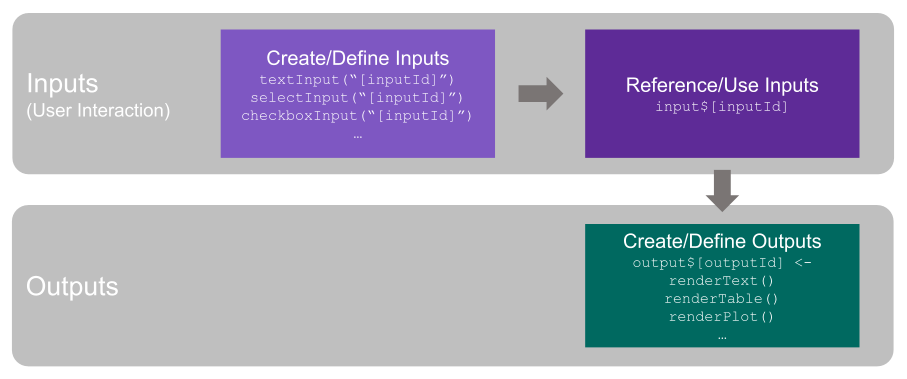
Inputs and Outputs

Let’s start with the basic idea of Shiny: it’s interactive. This means it’s got a stimulus/response paradigm at its core: the inputs are interactions by the user, and the outputs are the result of applying those inputs in some fashion.

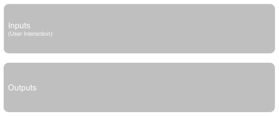
Creating the Inputs

The user interaction is through input controls, and the big (relatively speaking) decisions there are:

• What type of control is it (a checkbox, a dropdown, a slider, etc.)?
• What the options and default values are for the control
• The name of the control. This is the inputId that you specify and then reference elsewhere

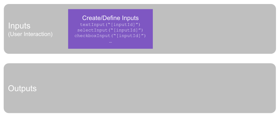
Referencing / Using the Inputs

Separate from creating the inputs, you then want to actually use the selected values from them. That’s a separate operation, and it’s an entirely different syntax—input$[inputId]—but, at its core, it’s linked back to the appropriate input using whatever inputId value you decided on when creating the input.

Creating Outputs

When it comes to the output—what you actually want to show the user as a result of their selections—things work similarly to inputs, but kind of in a reverse order.

You start by creating/defining the output. The two big things you have to do here are:

• Figure out the name you will use to refer to the output. This is the outputId and actually gets defined as output$[outputId] (this is the “similar…but in reverse” part when compared to inputs: you actually set the name by putting some value for outputId in output$[outputId]; remember that, for inputs, when using input$[inputId] you are simply referring to the inputId value you had already defined).

• Figure out the type of output you’re creating. Or, the type of output that you’re going to render. This winds up being defined using a render... function: renderPlot, renderText, etc. It’s a little tricky, in that you’re not actually displaying (rendering) anything with this. You are simply defining what will be rendered for the user in the next step.

The key here is that, since the output will be dynamic based on what the user has selected/set through the inputs, the inputs are actually used in the logic and code that defines the outputs. We’ll come back to that very shortly.

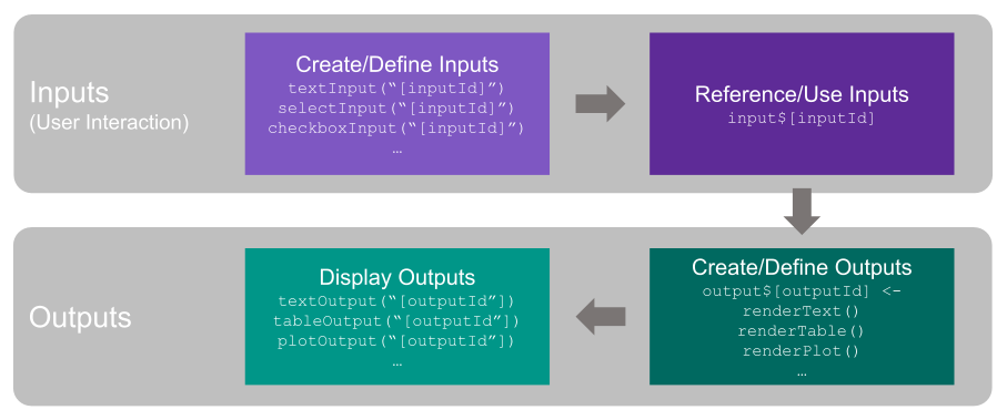
Display the Output

The last piece of the puzzle is actually displaying the resulting output to the user. This is accomplished using the ...Output("[outputId]) functions (textOutput(), plotOutput(), etc.). The primary argument for each of these functions is simply the outputId defined in the previous step.

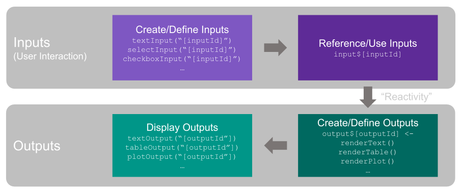
The Miracle of Reactivity

You simply cannot develop a healthy and satisfying relationship with Shiny without having a proper level of awe and appreciation for reactivity. You actually…can’t read very far on any documentation or tutorial about Shiny without hitting the topic pretty hard.

Functionally, reactivity is simply the link between the inputs and the outputs: when the user changes an input, all of the affected outputs will automatically reprocess and get updated. There are lots of tips and tricks for tweaking exactly what, how, and where reactivity comes into play. Those are important, but they are beyond the scope of this post. We can make one small addition to the diagram to reflect where reactivity sits (right between the inputs and outputs):

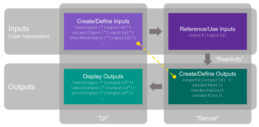
Front End and Back End

It’s useful to add one more layer to the diagram, and that is to recognize that, while we’ve been looking at it thus far as being two rows of operations, we can also think about it as two columns:

• The left column is actually the “front end.” It’s everything to do with the user interface. Or…in developer shorthand, the “UI.” And that’s why, in the early versions of Shiny, when you had to have two files for a single app, one of them was ui.R. That was “the left column.” In a “single file Shiny app,” you define a ui object (by convention) that then gets passed as the value for the ui argument in the shinyApp() function. In a flexdashboard file that is Shiny-enabled…the “UI” concept is just implicitly there, but is never explicitly referenced in the code.

• The right column is the “back end.” It’s where the actual crunching work happens—where the inputs get embedded into all manner of code so that useful outputs can be defined for rendering. You can think of this as being the “server” that’s doing the heavy lifting. You don’t have to think of it that way…but Shiny does! In a traditional, two-file Shiny app, the server.R file is where everything from the right column goes. In a single-file Shiny app, a server object typically gets defined and then used in the shinyApp() function as the value for the server argument. Again, in flexdashboard this distinction still exists, but it’s never explicitly referenced in the code.

And that’s really it.

Except…there’s just one more thing…

The Symmetry of Diagonal Definitions

It wasn’t until I started drawing up the diagram that I fully clicked on a few things. The “rows” (inputs vs outputs) and the “columns” (front end/UI vs. back end/server) were part of that. But there is one other piece that I referenced in passing earlier that I think bears calling out directly.

First, a quick reminder of two basic points:

• The first step for both inputs and outputs is defining them. That’s where you give them an ID—an inputId for inputs and an outputId for outputs.

• This definition occurs in the front end (the UI) for inputs and the back end (the server) for outputs

What’s interesting…but I realized can be a little confusing, even though it actually sorta’ makes sense, is that the underlying syntax for how those definitions are effected is quite different:

• Inputs have their inputId values defined as an argument inside a function (one of the ...Input() functions)

• Outputs have their outputId values defined as a value following the dollar sign in an output$... object definition

The definition of inputs and outputs are operations that occur in the “top left” and “bottom right” of our diagram, which, really, is why their syntax is so different.

I think (hope) this is helpful. It certainly has made the picture clearer in my mind as to how these four underlying components work together and how and why the specific syntax of each component falls as it does!